Code
library(tidyverse)
library(dplyr)
library(janitor)
library(MASS)
library(knitr)
library(kableExtra)Due to changing climate conditions, macroalgae coverage can impact the transitional phases in coral colonization. Because coral reefs play such a vital role in ecosystem services, understanding coral reef dynamics is important. One component of this is understanding how the macroalgae within these systems are being controlled. The herbivorous fishes Chlorurus sordidus, commonly known as parrot fish, and Ctenochaetus striatus, commonly known as striated surgeonfish, are essential reef fish species that feed directly on algae, therefore influencing the health of coral reefs.
Observation data was collected from coral reefs around Moʻorea, French Polynesia, at research stations LTER 1 and Resilience 2. Focal fish species were identified by a SCUBA diver, an estimated fish length (cm), the depth at the start and end of the observation period, substrate types, and the number of bites taken within 5 minutes was recorded. The data was collected over several days in July and August of 2010 between the times of 10:00 and 16:00, an identified period of time which corresponds to peak feeding rates for many herbivorous fishes (Adam, 2019).
Using this data, we want to understand how herbivore grazing bite counts are influenced by fish size, species, depth, and substrate.
library(tidyverse)
library(dplyr)
library(janitor)
library(MASS)
library(knitr)
library(kableExtra)# Load in the data.
data1 <- read_csv(here::here("posts",
"eds222-blog-post",
"data",
"MCR_LTER_HerbBite_Focal_Herb_Bite_Rates_2010_20120521.csv")) %>%
clean_names() %>%
dplyr::select(-c(time_period, depth_cat))
data2 <- read_csv(here::here("posts",
"eds222-blog-post",
"data",
"MCR_LTER_HerbBite_Addit_Bite_Rate_Data_2010_20120521.csv")) %>%
clean_names()
# Stacking the datasets and dropping unnecessary columns.
bite_data <- rbind(data1, data2) %>%
dplyr::select(-c("observer", "time_beg", "time_end", "stage", "notes")) %>%
drop_na()
# Creating a mean_depth column.
bite_data$mean_depth <- (bite_data$depth_beg + bite_data$dept_end) / 2
# Dropping the depth range columns.
bite_data <- bite_data %>%
dplyr::select(-c("depth_beg", "dept_end"))
# Of the substrate type create a column of the dominant substrate.
bite_data$dominant_substrate <- apply(
bite_data[, c("bare", "rubble", "cca", "sand", "other")],
1,
function(x) names(x)[which.max(x)])
# Drop individual substrate columns make species and substrates factors.
bite_data_clean <- bite_data %>%
dplyr::select(-c("bare", "rubble", "cca", "sand", "other")) %>%
mutate(species = factor(species),
dominant_substrate = factor(dominant_substrate))The data source provides two datasets that hold observational dat from different dates and locations in Moʻorea. After stacking the dataframes, columns that were not required for the analysis were dropped. Some cleaning of our variables was also conducted. A mean_depth column was created, which is the average depth during each observation. This was created by taking the average depth between the recorded depth at the start and end of the observation. A dominant_substrate column was also created, which represents the substrate that was bitten the most of all the possible substrates. This was done by detecting which substrate had the highest number of bites for each observed fish.
We’ll begin with basic data exploration by plotting fish body length (cm) and depth (ft) against the total bite count to visualize any potential relationships between these variables and our response variable, total number of bites. We also want to know the shape of the total bite count distribution to help determine what statistical model we should use for our analysis.
# Plot of size vs. total bites, by species.
ggplot(data = bite_data_clean, aes(x = size_cm, y = total_bites, color = species)) +
  geom_jitter() +
  labs(x = "Body Length (cm)",
       y = "Total Number of Bites",
       color = "Species") +
  scale_color_manual(values = c("dodgerblue", "violet"),
                     labels = c("Chlorurus sordidus (Parrotfish)",
                                "Ctenochaetus striatus (Striated surgeonfish)")) +
  theme_minimal()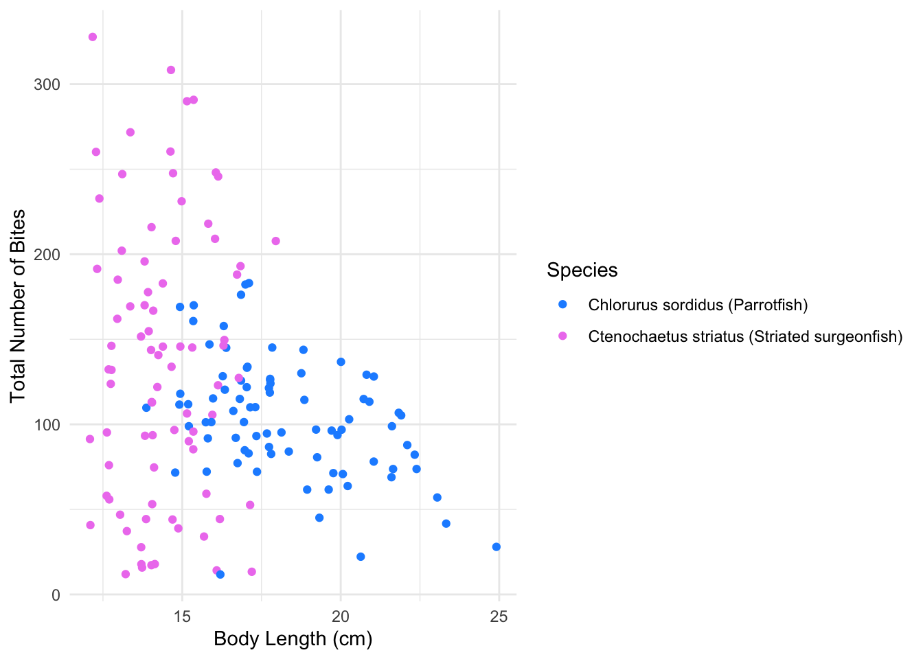
Figure 1 depicts differences in body length (cm) and total bite counts based on species. Striated surgeonfish have a wider range of body lengths (cm) compared to Parrotfish and display greater variability in total bite counts. Parrotfish body length (cm) and bite counts appear to be more clustered.
# Plot of mean depth vs. total bites, by species
ggplot(data = bite_data_clean, aes(x = mean_depth, y = total_bites, color = species)) +
  geom_jitter() +
  labs(x = "Mean Depth (ft)",
       y = "Total Number of Bites",
       color = "Species") +
  scale_color_manual(values = c("dodgerblue", "violet"),
                     labels = c("Chlorurus sordidus (Parrotfish)",
                                "Ctenochaetus striatus (Striated surgeonfish)")) +
  theme_minimal()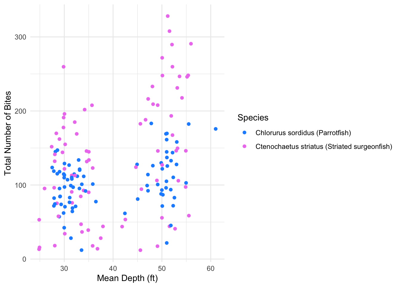
Figure 2 depicts greater variability and higher total bite counts for Striated surgeonfish. While parrotfish again seem to be more clustered around lower total bite counts.
# Total bite count distribution
ggplot(data = bite_data_clean, aes(x = total_bites)) +
  geom_histogram(binwidth = 10,
                 fill = "black") +
  labs(x = "Total Number of Bites",
       y = "Count") +
  theme_minimal()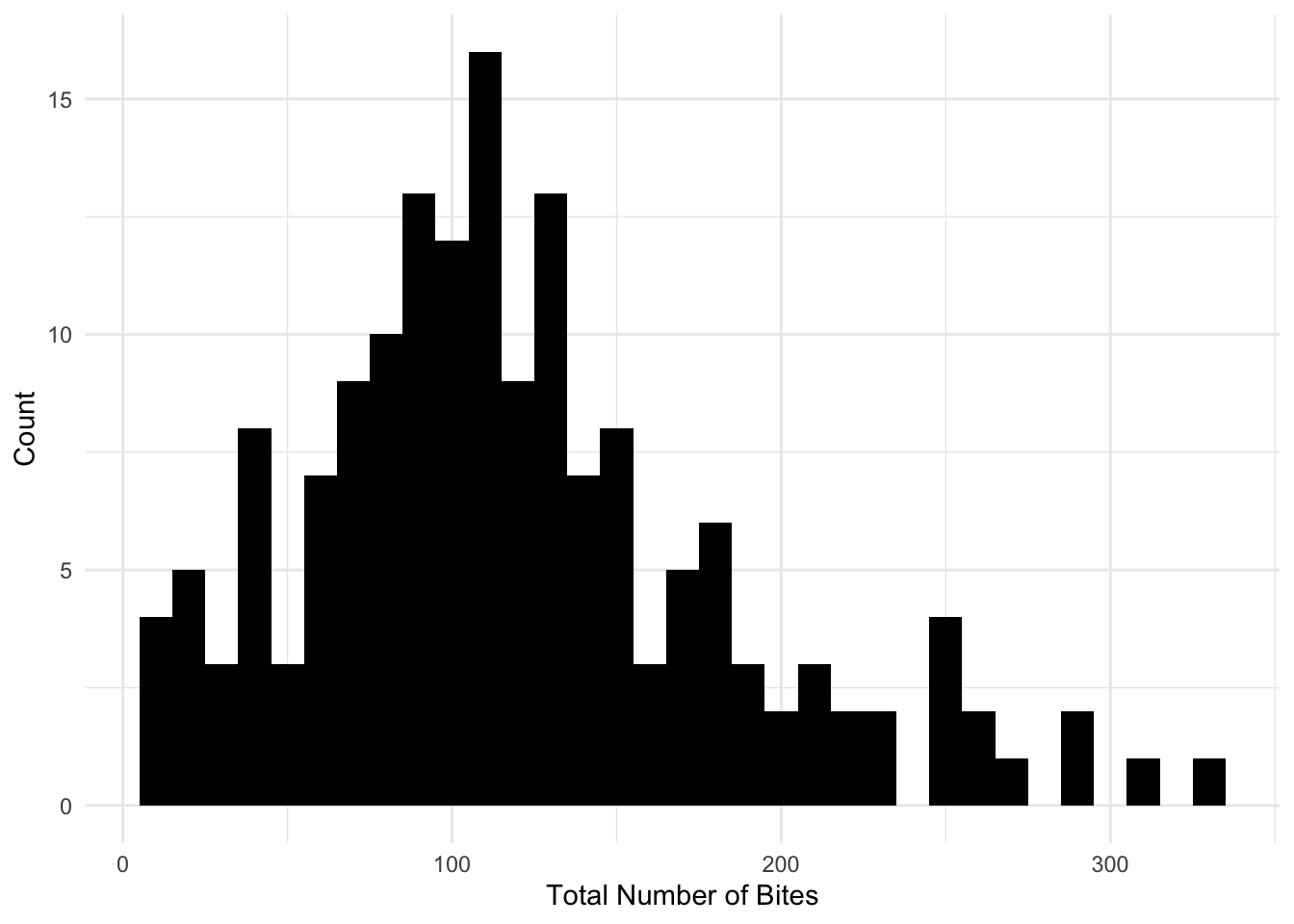
The data is not normally distributed. The total number of bites is right skewed, which can be indicative of overdispersion.
Research Question: How is the herbivore grazing bite counts related to fish size, species, depth, and substrate?
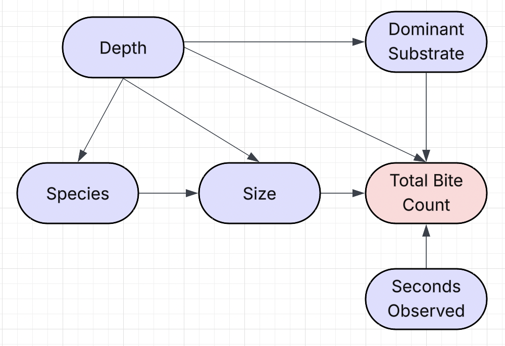
This DAG illustrates our hypothesized causal structure between predictors and the total bite counts. Depth directly affects dominant substrates, species, size, and total bite count. Species affects the total bite count through its effect on the size variable. Depth, dominant substrate, and size all influence total bite count. Observation time directly influences total bite count, but does not affect any other variable.
Null Hypothesis: Either size, species, depth, or substrate have no effect on bite count.
Alternative Hypothesis: A predictor/predictors have an effect on bite count.
Hypothesis in Statistical Notation:
\[H_0: \beta_i = 0 \\ H_A: \beta_i \neq 0\]
# Find the mean and variance.
var_total_bites <- var(bite_data_clean$total_bites)
mean_total_bites <- mean(bite_data_clean$total_bites)# Check that variance is greater than the mean.
if (var_total_bites > mean_total_bites) {
print("Calculations show that the variance of the `total_bites` is greater than the mean of `total_bites`.")
print(paste("Variance:", var_total_bites))
print(paste("Mean:", mean_total_bites))
}[1] "Calculations show that the variance of the `total_bites` is greater than the mean of `total_bites`."
[1] "Variance: 4127.29773305402"
[1] "Mean: 119.786585365854"What model?: Since we are dealing with count data our model options are Poisson Regression or Negative Binomial Regression. The Poisson distribution assumes that the mean and variance are equal, which is an assumption that our data does not meet. The mean of total_bites is 4127.2977331 and the variance of total_bites is 4127.2977331. Since the variance is greater than the mean, the distribution of our count data, total_bites, exhibits overdispersion, which is a factor that the Negative Binomial Regression model accounts for.
\[ \begin{aligned} \text{BiteCount} &\sim Negative Binomial(\mu, \theta) \\ log(\mu) &= \beta_0 + \beta_1 \text{Size} + \beta_2 \text{Species} + \beta_3 \text{Depth} + \beta_4 \text{Substrate} \\ \end{aligned} \]
Before fitting the Negative Binomial Regression model to our real data, we can fit the model to simulated data generated from the coefficients and parameters we define. Using these values, we can generate data from these values to see if we are able to successfully backtrack our defined coefficients through fitting the Negative Binomial Regression model. This process ensures that our code to model the Negative Binomial Regression is implemented correctly with the appropriate parameters, and both the link function and the response space are used properly.
# Set seed for reproducibility purposes.
set.seed(123)

# Select coefficient values.
beta0 <- 1
beta1 <- -0.3
theta <- 1.5

# Generate random x values.
x1 <- rnorm(10000, mean = 0, sd = 2)

# Find mu in link space.
log_mu <- beta0 + beta1 * x1

# Transform the log_mu to response space.
mu <- exp(log_mu)

# Generate random y values.
y <- rnbinom(n = 10000, size = theta, mu = mu)

# Create a tibble of x1 and y.
sim_data <- tibble(x1, y)

# Fit a negative binomial model to the simulated data.
negbi_sim <- glm.nb(y ~ x1, data = sim_data)

beta0_sim <- coef(negbi_sim)[1]
beta1_sim <- coef(negbi_sim)[2]
theta_sim <- negbi_sim$theta# Create a table to compare defined and simulated values
sim_table <- tibble(
Parameter = c("β<sub>0</sub>", "β<sub>1</sub>", "θ"),
Set_Value = c(beta0, beta1, theta),
Simulated_Value = round(c(beta0_sim, beta1_sim, theta_sim), 2)) %>%
rename("Parameter" = Parameter,
"Defined Value" = Set_Value,
"Simulated Value" = Simulated_Value) %>%
kbl(escape = FALSE,
caption = "Table 1: Comparing defined parameters to simulated paramters") %>%
kable_paper(full_width=TRUE)
sim_table| Parameter | Defined Value | Simulated Value |
|---|---|---|
| β0 | 1.0 | 1.00 |
| β1 | -0.3 | -0.29 |
| θ | 1.5 | 1.49 |
After fitting our simulated data, we can see that the coefficients are very similar to the values that we defined. This means that our process for implementing a Negative Binomial Regression model on data is correct, and we can therefore apply this to our actual bite count data from Moʻorea.
We’ll use and additive Negative Binomial Regression model. Our predictor variables are size_cm, species, mean_depth, dominant_substrate, and an offset of seconds_observed.
What is an offset?: An offset variable represents the size, exposure or measurement time, or population size of each observational unit (Parry, 2018). Within this study the offset variable is seconds_observed, where the coefficient for seconds_observed is constrained to be 1, meaning that the model will represent rates rather than counts.
Why use an offset?: Observations were conducted within a 300-second window, resulting in some variability within the amount of time spent observing individual fishes, as seen in Figure 5. When using an offset, the assumption is made that doubling the unit size (seconds observed) will lead to a doubling of the count outcome. In the case of bite counts, more count data could be collected in a larger time window (300 seconds) compared to a smaller one (200 seconds). In summary, the offset ensures that genuinely high bite count occurrence is distinguished from high bite counts that result from larger time windows.
# Seconds observed distribution.
ggplot(data = bite_data_clean, aes(x = seconds_observed)) +
  geom_histogram(binwidth = 20,
                 fill = "black") +
  labs(x = "Seconds Observed",
       y = "Count of Observations") +
  theme_minimal()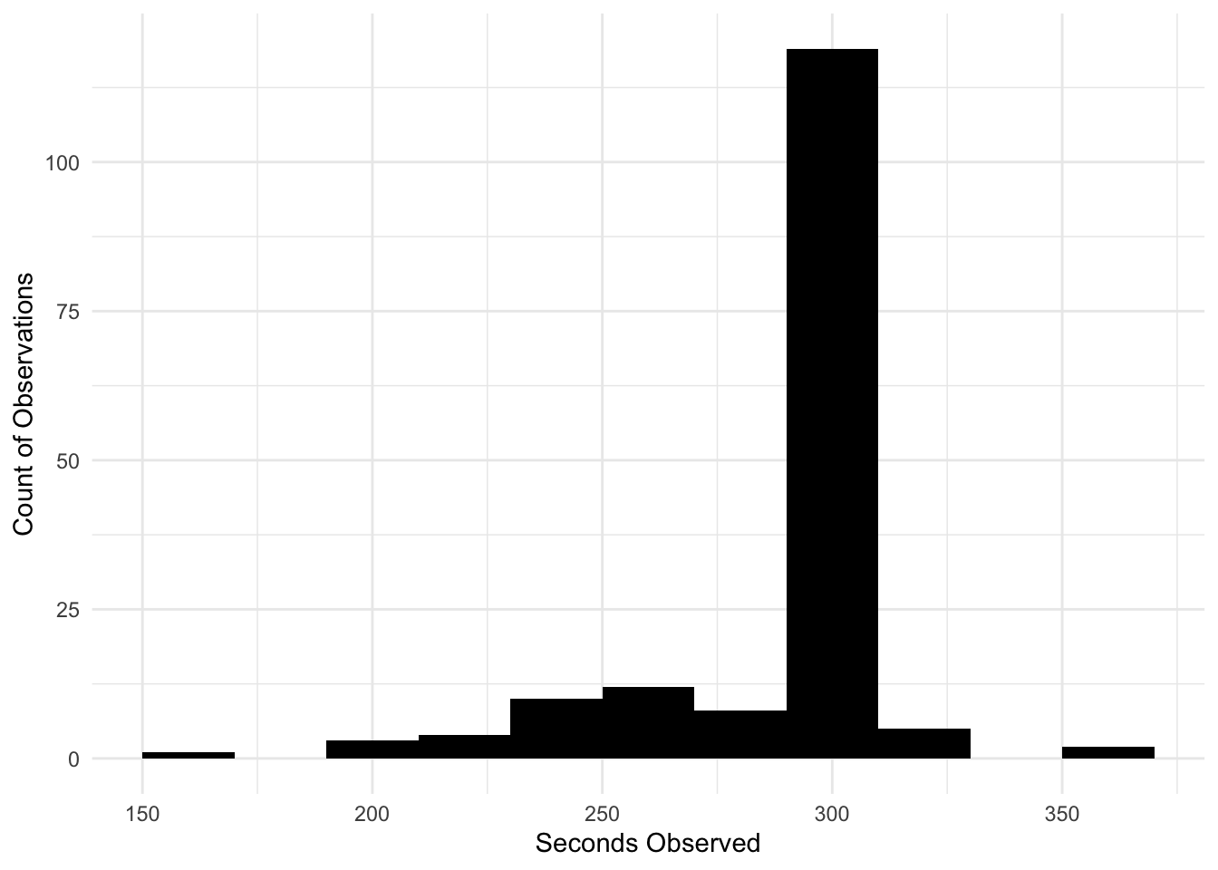
\[ \begin{aligned} \text{BiteCount} &\sim Negative Binomial(\mu, \theta) \\ log(\mu) &= \beta_0 + \beta_1 \text{Size} + \beta_2 \text{Species} + \beta_3 \text{Depth} + \beta_4 \text{Substrate} \\ \end{aligned} \]
# Fitting a additive Negative Binomial Regression model.
full_model <- glm.nb(total_bites ~ size_cm + species + mean_depth + dominant_substrate + offset(log(seconds_observed)), data = bite_data_clean)# Create a table of the coefficients.
full_model_table <- broom::tidy(full_model) %>%
kbl(caption = "Table 2: Coefficient Estimates of the Full Additive Model") %>%
kable_paper(full_width=TRUE)
full_model_table| term | estimate | std.error | statistic | p.value |
|---|---|---|---|---|
| (Intercept) | -0.7224262 | 0.4229417 | -1.7080987 | 0.0876180 |
| size_cm | -0.0519902 | 0.0215223 | -2.4156482 | 0.0157072 |
| speciesCtenochaetus striatus | 0.0947912 | 0.1189715 | 0.7967551 | 0.4255933 |
| mean_depth | 0.0152081 | 0.0044205 | 3.4403547 | 0.0005810 |
| dominant_substraterubble | 0.0594797 | 0.1318579 | 0.4510897 | 0.6519249 |
The model summary tells us:
Size has a negative and statistically significant effect, indicating that when other variables are held constant, larger fish tend to have lower expected bite rates; when holding other predictor variables constant.
The species effect, with parrot fish being our reference level, is not statistically significant, indicating that the expected bite count between the two species are statistically the same, when holding other predictor variables constant.
Depth is a statistically significant predictor as our p-value is less than 0.001. Therefore, depth has a statistically significant positive effect, meaning that at greater depths we expect higher bite rates, when other variables are held constant.
The substrate effect, with bare being the reference level, is not significant. This means that substrate does not statistically influence expected bite counts.
In summary, bite count decreases when fish length increases, suggesting that larger fish take fewer bites, which can be explained by the idea of larger fish taking less bites, due to taking bigger bites. Bite counts also significantly increase as depth increases. This can indicate more food availability at different depth levels.
Next I’ll generate expected bite count predictions. The predictions will be generated varying the body lengths (cm), size_cm, and holding all other variables constant.
# Create grid for generated predictions.
bite_pred_grid <- expand_grid(
  size_cm = seq(12, 25, by = 0.5),
  mean_depth = mean(bite_data_clean$mean_depth),
  species = levels(bite_data_clean$species),
  seconds_observed = mean(bite_data_clean$seconds_observed)) %>%
  mutate(
    species = factor(species, levels = levels(bite_data_clean$species)),
    dominant_substrate = factor("bare", levels = levels(bite_data_clean$dominant_substrate)))

# Generate predictions.
bite_pred_grid$predicted_bites <- predict(full_model,
                                          newdata = bite_pred_grid,
                                          type = "response")

# Generate a standard error for predictions.
bite_pred_se <- predict(object = full_model,
                        newdata = bite_pred_grid,
                        type = "link",
                        se.fit = TRUE)

# Go from link space to response space
linkinv <- family(full_model)$linkinv
bite_pred_grid <- bite_pred_grid %>%
  mutate(

    # get log(mu)
    log_mu = bite_pred_se$fit,

    # 95% CI in link space
    log_mu_se = bite_pred_se$se.fit,
    log_mu_lwr = qnorm(0.025, mean = log_mu, sd = log_mu_se),
    log_mu_upr = qnorm(0.975, mean = log_mu, sd = log_mu_se),

    # undo the link function using linkinv
    mu = linkinv(log_mu),
    mu_lwr = linkinv(log_mu_lwr),
    mu_upr = linkinv(log_mu_upr)
  )
The expected bite count predictions were generated in response space, while the 95% confidence interval for the expected bite count predictions were generated in link space.
We’ll then plot the expected bite count predictions along with the observed values to see how well our predicted expected values generated from the additive model, fit the data.
# Plot the observed variables and
ggplot(bite_pred_grid, aes(size_cm, predicted_bites, color = species)) +
  geom_ribbon(aes(ymin = mu_lwr, ymax = mu_upr), alpha = 0.2) +
  geom_line() +
  geom_jitter(data = bite_data_clean, aes(x= size_cm, y = total_bites)) +
  scale_color_manual(values = c("dodgerblue", "violet"),
                     labels = c("Chlorurus sordidus (Parrotfish)",
                                "Ctenochaetus striatus (Striated surgeonfish)")) +
  facet_wrap(~species, scales = "free_x") +
  labs(x = "Body Length (cm)",
       y = "Total Bite Counts",
       color = "Species") +
  theme_minimal()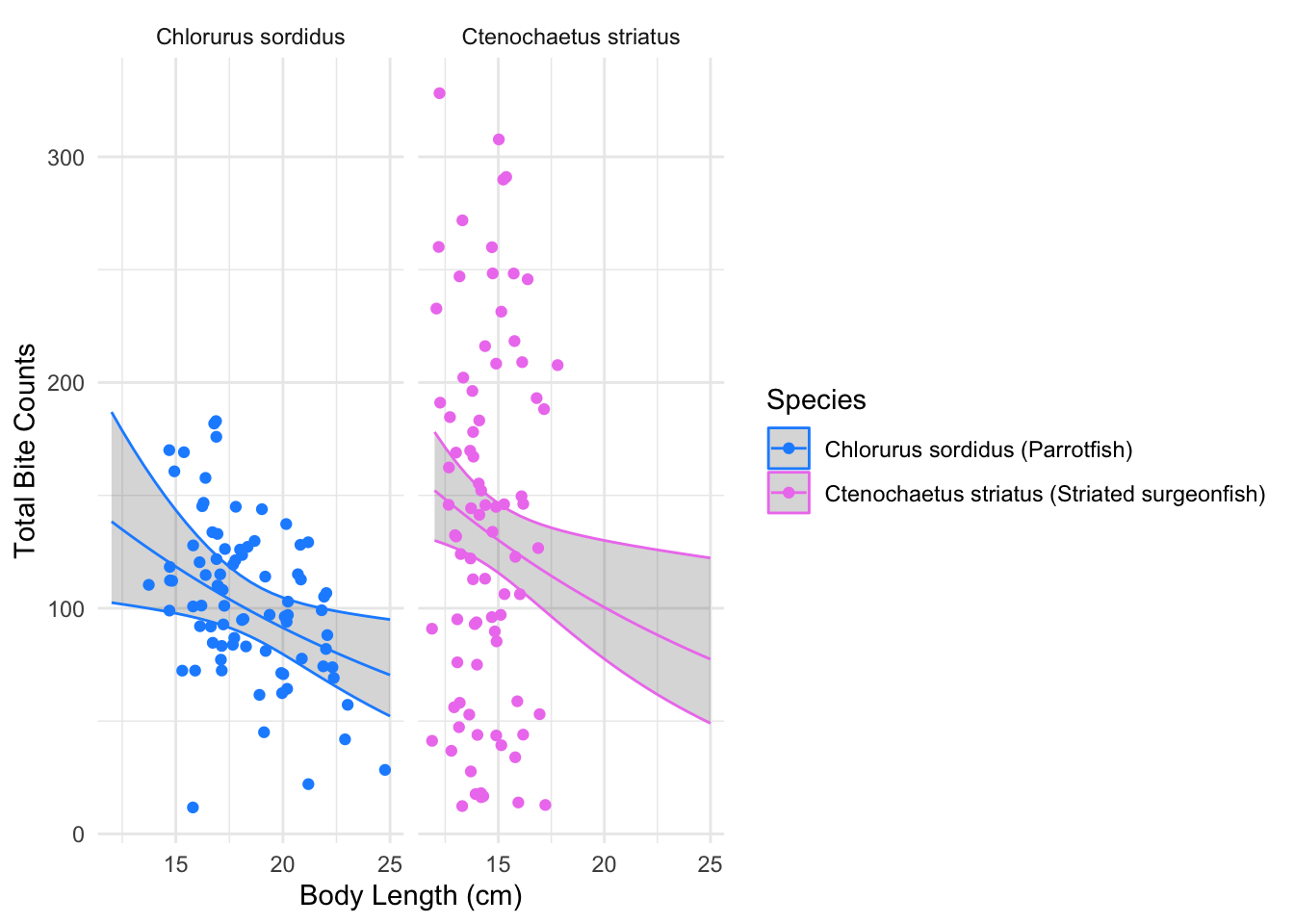
The figure displays the relationship between the length of the fish (cm) and total bite counts for parrotfish and striated surgeonfish, overlaid with predicted expected bite counts generated from the additive Negative Binomial Regression model. The 95% confidence interval is represented as the shaded grey region.
Connecting Coefficient Estimates to Predicted Bite Rates:
Recall our size effect coefficient interpretation: “Size has a negative and statistically significant effect, indicating that when other variables are held constant, larger fish tend to have lower expected bite rates; when holding other predictor variables constant.”
When generating predictions of expected bite counts, we varied our size variable and held all the other predictor variables constant. By doing so, we should be able to visualize the size effect within our predicted expected values.
For both parrotfish and striated surgeonfish, the predicted expected bite count slope curves downward as size increases. Indicating that larger fish tend to have lower bite rates, which attests to the statistically significant negative coefficient for the size effect in the model.
Since depth showed a statistically significant positive effect in the additive model above, I wanted to test whether this effect was consistent between the species. A species x depth interaction within the Negative Binomial Regression model will detect if the relationship between depth and bite rate differs among the two species.
\[ \begin{aligned} \text{BiteCount} &\sim Negative Binomial(\mu, \theta) \\ log(\mu) &= \beta_0 + \beta_1 \text{Size} + \beta_2 \text{Species} + \beta_3 \text{Depth} + \beta_4 \text{(Species x Depth)} + \beta_5{Substrate} \\ \end{aligned} \]
# Fitting a additive Negative Binomial Regression model.
final_model <- glm.nb(total_bites ~ size_cm + species*mean_depth + dominant_substrate + offset(log(seconds_observed)), data = bite_data_clean)# Create a coefficient summary table.
final_model_table <- broom::tidy(final_model) %>%
kbl(caption = "Table 3: Coefficient Estimates of the Full Additive-Interactive Model") %>%
kable_paper(full_width=TRUE)
final_model_table| term | estimate | std.error | statistic | p.value |
|---|---|---|---|---|
| (Intercept) | -0.1330416 | 0.4784270 | -0.2780812 | 0.7809500 |
| size_cm | -0.0647547 | 0.0215775 | -3.0010257 | 0.0026907 |
| speciesCtenochaetus striatus | -0.6869812 | 0.3583561 | -1.9170349 | 0.0552335 |
| mean_depth | 0.0061290 | 0.0060036 | 1.0208837 | 0.3073096 |
| dominant_substraterubble | 0.0546794 | 0.1300324 | 0.4205060 | 0.6741159 |
| speciesCtenochaetus striatus:mean_depth | 0.0183200 | 0.0080984 | 2.2621793 | 0.0236863 |
Size again has a statistically significant negative effect, indicating that when other variables are held constant, larger fish tend to have lower expected bite rates.
The species effect represents the difference in expected bite counts between the species, when the depth is 0. Therefore, when depth is 0, we’d expect striated surgeonfish to have lower expected bite rated than parrotfish. However, this effect could be considered not statistically significant as it’s p-value is 0.055.
The depth effect on parrot fish, is not significant. Meaning that depth does not affect the expected bite count of parrotfish.
The dominant substrate effect is again not significant. Therefore, when holding all other variables constant, substrate does not affect the expected bite count.
The interaction between species and depth effect, represents the differing bite rates between parrotfish and striated surgeonfish because of depth effect. The interaction has a positive, statistically significant effect, indicating that striated surgeon fish experience a stronger increase in expected bite rates with increasing depth, compared to parrotfish (reference species).
In summary, this new additive-interaction Negative Binomial Regression model indicates that again larger fish take less bites. Within this new model an important effect is that at deeper depths, there is a stronger increase in the expected bite counts of striated surgeon fish compared to parrotfish. Therefore, the model reveals different behaviors and patterns within species related to herbivory grazing upon coral reefs.
Finally, we’ll generate expected bite count predictions from the new additive-interactive Negative Binomial Regression model. The predictions will be generated varying the depth, mean_depth, and holding all other variables constant.
# Find the mean size, by species.
species_means <- bite_data_clean %>%
  group_by(species) %>%
  summarise(
    mean_size = mean(size_cm, na.rm = TRUE))

# Create grid for generated predictions.
bite_pred_grid2 <- expand_grid(
  mean_depth = seq(25, 61, by = 0.5),
  species = levels(bite_data_clean$species),
  seconds_observed = mean(bite_data_clean$seconds_observed)) %>%
  left_join(species_means, by = "species") %>%
  mutate(
    size_cm = mean_size,
    dominant_substrate = factor("bare", levels = levels(bite_data_clean$dominant_substrate)),
    species = factor(species, levels = levels(bite_data_clean$species)))

# Generate predictions.
bite_pred_grid2$predicted_bites <- predict(final_model,
                                          newdata = bite_pred_grid2,
                                          type = "response")

# Generate a standard error for predictions.
bite_pred_se2 <- predict(object = final_model,
                        newdata = bite_pred_grid2,
                        type = "link",
                        se.fit = TRUE)

# Go from link space to response space
linkinv <- family(final_model)$linkinv
bite_pred_grid2 <- bite_pred_grid2 %>%
  mutate(
    # get log(mu)
    log_mu = bite_pred_se2$fit,
    # 95% CI in link space
    log_mu_se = bite_pred_se2$se.fit,

    log_mu_lwr = qnorm(0.025, mean = log_mu, sd = log_mu_se),
    log_mu_upr = qnorm(0.975, mean = log_mu, sd = log_mu_se),

    # undo the link function using linkinv
    mu = linkinv(log_mu),
    mu_lwr = linkinv(log_mu_lwr),
    mu_upr = linkinv(log_mu_upr)
  )
The expected bite count predictions were, again, generated in response space, while the 95% confidence interval for the expected bite count predictions were generated in link space.
We’ll then plot the expected bite count predictions along with the observed values to see how well our predicted expected values generated from the additive-interactive model, fit the data.
# Plot the observed variables and
ggplot(bite_pred_grid2, aes(mean_depth, predicted_bites, color = species)) +
  geom_ribbon(aes(ymin = mu_lwr, ymax = mu_upr), alpha = 0.2) +
  geom_line() +
  geom_jitter(data = bite_data_clean, aes(x= mean_depth, y = total_bites)) +
  scale_color_manual(values = c("dodgerblue", "violet"),
                     labels = c("Chlorurus sordidus (Parrotfish)",
                                "Ctenochaetus striatus (Striated surgeonfish)")) +
  facet_wrap(~species, scales = "free_x") +
  labs(x = "Depth (ft)",
       y = "Total Bite Counts",
       color = "Species") +
  theme_minimal()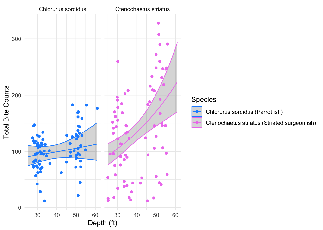
The figure displays the relationship between the depth (ft) and total bite counts for parrotfish and striated surgeonfish, overlaid with predicted expected bite counts generated from the additive-interactive Negative Binomial Regression model. The 95% confidence interval is represented as the shaded grey region.
Connecting Coefficient Estimates to Predicted Bite Rates:
Recall our species x depth interaction effect coefficient interpretation: “The interaction between species and depth effect represents the differing bite rates between parrotfish and striated surgeonfish because of the depth effect. The interaction has a positive, statistically significant effect, indicating that striated surgeon fish experience a stronger increase in expected bite rates with increasing depth, compared to parrotfish (reference species).”
When generating predictions of expected bite counts, we varied our depth variable and held all the other predictor variables constant. By doing so, we should be able to visualize the interaction between species and depth effect within our predicted expected values.
For both parrotfish and striated surgeonfish, the predicted expected bite counts slope curves upward as depth increases. However, as depth increases, the upward curve of the slope is steeper for striated surgeon fish. Indicating that striated surgeon fish experience a stronger increase in expected bite rates with increasing depth, compared to parrotfish. This aligns with the statistically significant positive coefficient for the depth and species interaction effect in the additive-interactive model.
Referring back to our hypothesis:
Null Hypothesis: Either size, species, depth, or substrate have no effect on bite count.
Alternative Hypothesis: A predictor/predictors have an effect on bite count.
Hypothesis in Statistical Notation:
\[H_0: \beta_i = 0 \\ H_A: \beta_i \neq 0\]
From the additive Negative Binomial Regression model, are statistically significant effects on total bite count were size and depth. Therefore, we would reject the null hypothesis that the predictor size or depth have no effect on bite count. The additive model provides evidence that the relationship between these predictors and total bite count is not due to chance.
From the additive-interactive Negative Binomial Regression model, are statistically significant effects on total bite count were size and the species x depth interaction. Therefore, we would reject the null hypothesis that the predictors size and depth have no effect on bite count. Again, the additive-interactive model provides evidence that the relationship between these predictors and total bite count is not due to chance.
From this analysis, we found that size has a significant effect on total bite counts, where larger fish take fewer bites. Another significant finding was that there was a significant effect of the interaction of species and depth. This indicates that there are different feeding behaviors of the species at different depths. After collecting these results, further research can be done to understand the behaviors of the species at different depths, which would include collecting other variables that could have an effect on bite counts. Such as different environmental factors, such as temperature, pH levels, presence of other species, etc. This analysis could provide a baseline for stakeholders when it comes to conservation decision-making. For example, by using this analysis and with further research, size limits can be created or updated to protect the size range of species that feed the most on the coral reefs.
Holbrook, S., Schmitt, R., Adam, T. et al. Coral Reef Resilience, Tipping Points and the Strength of Herbivory. Sci Rep 6, 35817 (2016). https://doi.org/10.1038/srep35817
Moorea Coral Reef LTER and T. Adam. 2019. MCR LTER: Coral Reef Resilience: Herbivore Bite Rates on the North Shore Forereef July-August 2010 ver 2. Environmental Data Initiative. https://doi.org/10.6073/pasta/5a6798c5694d5a58362ab42e584b7b71 (Accessed 2025-12-04).
Parry, S. (2018, March). To Offset or Not: Using Offsets in Count Models. Https://Cscu.cornell.edu/; Cornell Statistical Consulting Unit. https://cscu.cornell.edu/wp-content/uploads/offsets.pdf
@online{miura2025,
  author = {Miura, Jaslyn},
  title = {Grazing {Patterns} of {Herbivorous} {Fish} in {Moʻorea}},
  date = {2025-12-11},
  url = {https://jaslynmiura.github.io/posts/eds222-blog-post/},
  langid = {en}
}